Quick-start tutorial

Kriging, DACE modelling, and Gaussian-process emulation may all be considered to be applications of curve fitting. And in this respect, curve fitting is the principal intended use of PyMimic. In this quick-start tutorial we will fit a curve to some user-generated data.

Basic use of PyMimic for curve-fitting

Suppose that we have some data, which, for the sake of concreteness, we take to be a noisy sample of the Forrester function, \(f: [0, 1] \longrightarrow \mathbf{R}\) [F08], given by

\[x(t) = (6t - 2)^{2}\sin(12t - 4),\]

namely \((t_{i}, x(t_{i}) + \epsilon_{i})_{i = 1}^{n}\), where \(\epsilon_{i}\) is the error associated with the \(i\)-th element of the sample. We may fit a curve to this data using either the best linear predictor (BLP) or the best linear unbiased predictor (BLUP). First we must generate the sample. Second we must use this sample to predict the value of the Forrester function for some arbitrary argument, \(t_{*} \in [0, 1]\).

First, then, generate the sample. The Forrester function is included in PyMimic’s testfunc module, so we do not need to define it ourselves. We will use Gaussian errors, though Gaussian errors are not necessary.

>>> import numpy as np
>>> import pymimic as mim
>>> ttrain = np.linspace(0., 1., 10)
>>> xtrain = mim.testfunc.forrester(ttrain) + 0.5*np.random.randn(10)

The Best linear unbiased predictor

Let us fit a curve to the data using the BLUP. Using our sample we now initialize an instance of the class Blup. In order to do this, we must specify a second-moment kernel. By default, PyMimic uses the squared-exponential kernel.

>>> blup = mim.Blup(ttrain, xtrain, var_error=0.5**2.))

Note that we have passed the variance of the error to Blup, and not the standard deviation.

Now tune the emulator using the class’s optimization method.

>>> blup.opt()
   direc: array([[-4.71202552e-03,  2.63909305e-03],
                 [-9.97534341e-05,  6.29293728e-04]])
     fun: 36.52459551952859
 message: 'Optimization terminated successfully.'
    nfev: 291
     nit: 9
  status: 0
 success: True
       x: array([1.55841236, 0.6449727 ])

(For an explanation of this output, see Optimization.) Note that the parameter of the second-moment kernel has been set to its maximum-likelihood estimate. This is stored as the attribute args.

>>> blup.args
(80.74538835868711, 31.626405926933707)

Now predict the value of the Forrester function, \(x(t_{*})\), for some random element of the domain, \(t_{*}\). This is done by the class method xtest(), which returns both the prediction and the mean-squared error of that prediction.

>>> t = np.random.rand()
>>> blup.xtest(t)
(array(-5.14655856), array(0.36967169))

We may compare the prediction with \(x(t_{*})\).

>>> mim.testfunc.forrester(t)
-5.561076962415382

We are not limited to computing one prediction at a time. In fact, we may compute any number of predictions. Let us generate 50 predictions and their mean-squared errors, spaced evenly across the Forrester function’s domain. We will assign these to variables, x and mse, so that we can continue to use them.

>>> t = np.linspace(0., 1.)
>>> x, mse = blup.xtest(t)

Now plot the predictions along with the true values of the function. First, plot the predictions, and their three-sigma prediction intervals.

>>> import matplotlib.pyplot as plt
>>> plt.plot(t, x)
>>> plt.fill_between(t, x - 3.*np.sqrt(mse), x + 3.*np.sqrt(mse))
>>> x_forrester = mim.testfunc.forrester(t)
>>> plt.plot(t, x_forrester)
>>> plt.scatter(ttrain, xtrain)

We get the plot shown in Fig. 1.

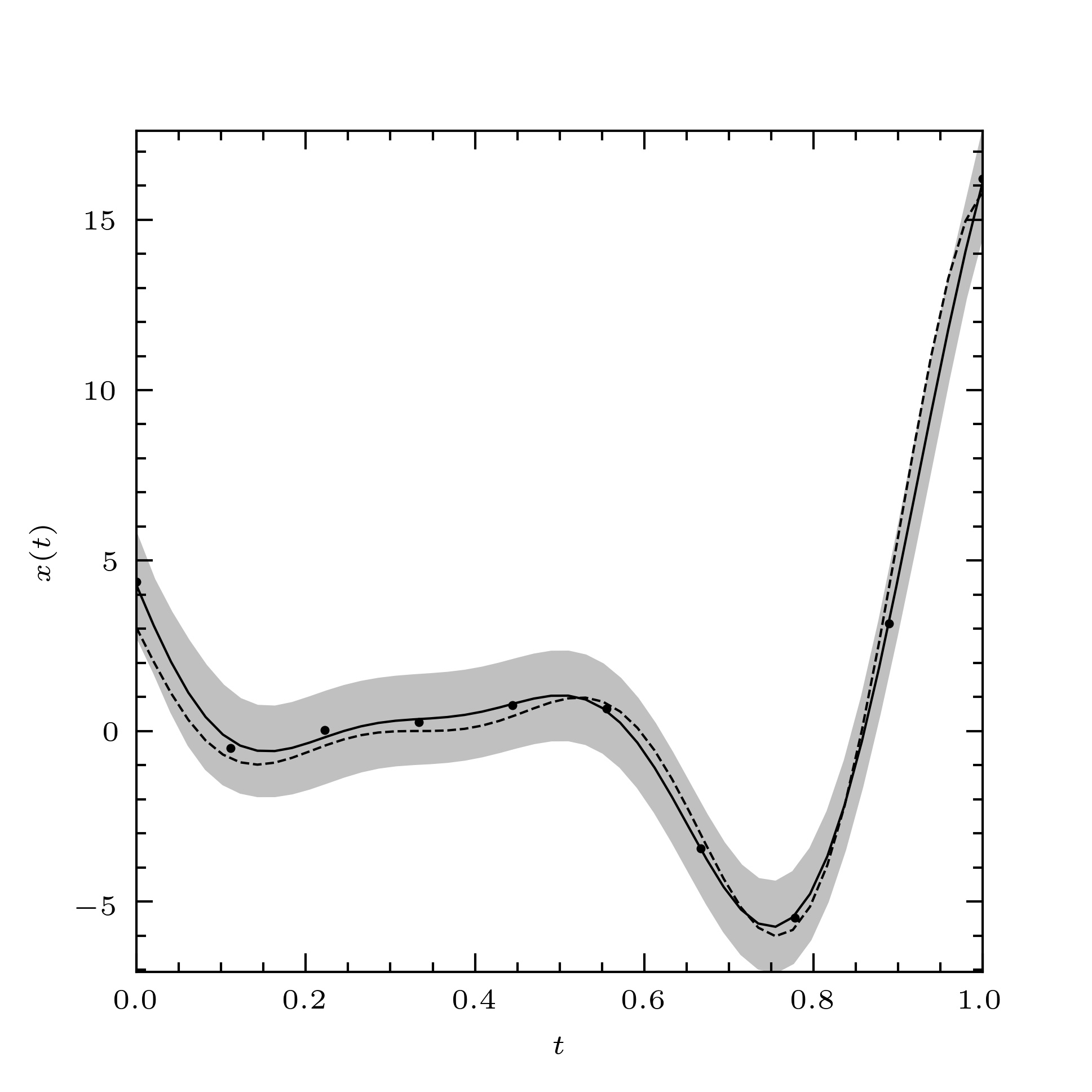
Fig. 1 The Forrester function (dashed line), a noisy sample of the Forrester function (filled circles) and a curve fitted to this sample using the BLUP (solid line). The three-sigma prediction interval for the fitted curve is also shown (solid grey band).

In general we are not able to compare the fitted curve directly with the function underlying our data. Instead, we may assess the performance of a fitted curve using leave-one-out cross-validation. The leave-one-out cross-validation residuals and their variance may be obtained as follows.

>>> blup.loocv
(array([ 4.52392036, -2.19276424,  1.13209079, -0.37317826, -0.36070607,
         0.42370805,  0.05501436, -0.55527947, -0.394956  ,  4.57205699]),
 array([13.04227266,  3.0432301 ,  1.92073694,  1.73096003,  1.73091835,
         1.73091835,  1.73096003,  1.92073694,  3.0432301 , 13.04227266]))

We may plot these as follows to give us Fig. 2.

>>> mim.plot.diagnostic(xtrain, *blup.loocv)

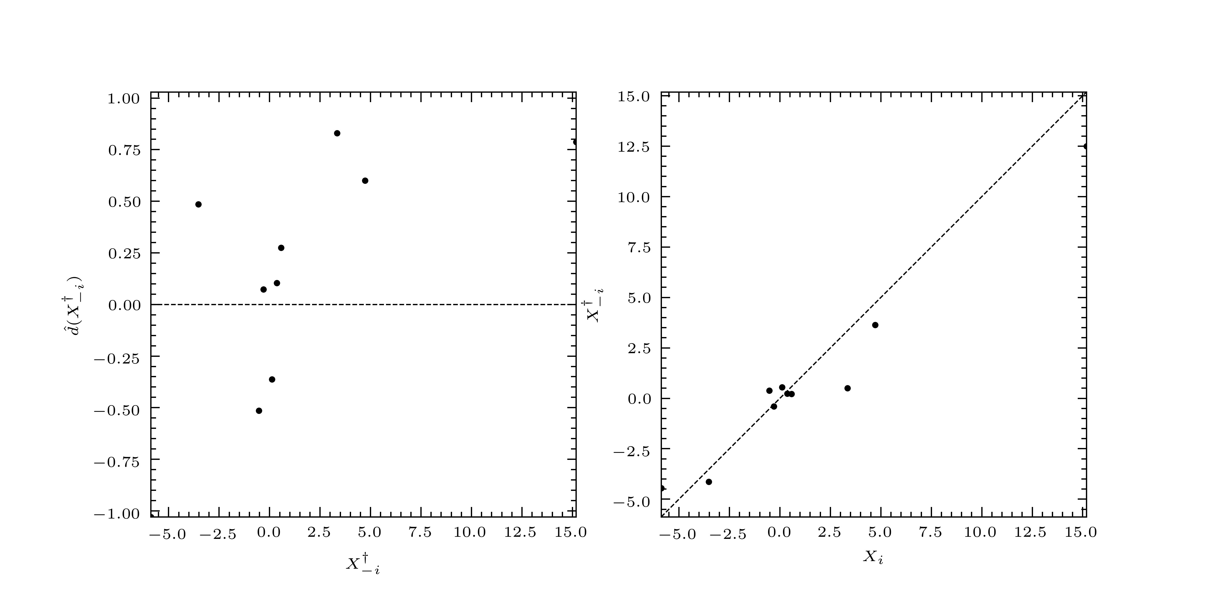
Fig. 2 The standardized leave-one-out residuals (left), and leave-one-out predictors (right).

The standardized leave-one-out residuals are small and randomly distributed so we say, in this case, that the predictor has passed validation, and that we may trust the fitted curve and its associated prediction interval.

The best linear predictor

We may fit a curve to the data using the BLP in exactly the same way. Instead of using the class Blup, we use the class Blp.

Kriging and emulation

In the case of vanishing obervational errors, the BLP and BLUP may be used as interpolators. In the field of geostatistics the use of such interpolators to construct maps of geological features is known as 'Kriging' [C86]. In computer science the use of such interpolators to construct metamodels of expensive simulations is known as 'DACE modelling' [S89] or 'Gaussian-process emulation' [RW06].

References

[F08]

Forrester, A., Sobester, A., and A. Keane. 2008. Engineering design via surrogate modelling: a practical guide. Chichester: Wiley.

[C86]

Cressie, N. 1986. ‘Kriging nonstationary data’ in Journal of the American Statistical Association, 81 (395): 625–34. Available at https://www.doi.org/10.1080/01621459.1986.10478315.

[RW06]

Rasmussen, C.E., and C.K.I. Williams. 2006. Gaussian processes for machine learning. Cambridge: MIT Press.

[S89]

Sacks, J., Welch, W. J., Mitchell, T.J., and H. P. Wynn. 1989. ‘Design and analysis of computer experiments’ in Statistical science, 4 (4): 409–23. Available at https://www.doi.org/10.1214/ss/1177012413.