PyMimic package
pymimic.basis module
A suite of basis functions
A suite of bases for spaces of mean-value functions (parameter
basis in the class pymimic.emulator.Blup)
-
pymimic.basis.const()[source]¶ Return a tuple consisting of the constantly one function
The constantly one function is the function \(f:\mathbf{R}^{n} \longrightarrow \mathbf{R}\) given by
\[f(t) = 1.\]- Returns:
res – A tuple consisting of the constantly one function
- Return type:
(1,) tuple
Example
Generate a basis:
>>> pymimic.basis.const()
(<function const.<locals>.fun at 0x7f800305cc80,)
Evaluate elements of the tuple for one one-dimensional argument:
>>> pymimic.basis.const()[0](0.)
array(1.)
Evaluate elements of the tuple for two one-dimensional arguments:
>>> pymimic.basis.const()[0]([0., 1.])
array([1., 1.])
Evaluate elements of the tuple for one two-dimensional argument:
>>> pymimic.basis.const()[0]([[0., 1.]])
array(1.)
Evaluate elements of the tuple for two two-dimensional arguments:
>>> pymimic.basis.const()[0]([[0., 1.], [2., 3.]])
array([1., 1.])
pymimic.design module
Experimental design module for PyMimic
This module provides the design() function for use in generating
experimental designs.
-
pymimic.design.design(bounds, method='lhs', n=None)[source]¶ Return an experimental design.
Let \(X\) be a real-valued random process, indexed by the set \(T\), a compact rectangular region of \(\mathbf{R}^{d}\). An experimental design of size \(n\) is a set of \(n\) elements of this region.
- Parameters:
bounds ((d, 2) array-like) – Bounds of design.
method (str, optional) –
Sample method. This may be one of:
"lhs"(\(2 \leq d \leq 10\) and \(d < n \leq 100\), \(n = 10d\) by default) Latin-hypersquare design;"gmlhs"(\(2 \leq d \leq 10\) and \(d < n \leq 100\), \(n = 10d\) by default) generalized Latin-hypersquare design;"random"(\(n = 10d\) by default) random design; or"regular"(\(n = 10\) by default) regular-lattice design.
The default is
"lhs".n (int, optional) – Size of design. The default value is dependent on the design method.
- Returns:
design – Design.
- Return type:
(n, d) ndarray
Notes
Latin-hypersquare designs are read from look-up tables, generated using the method of maximum projection [JB15, BJ18]. They are then permuted using a randomly chosen hyperoctohedral transformation.
References
[M79]McKay, M. D., Beckman, R. J., and W. J. Conover. 1979. 'A comparison of three methods for selecting values of input variables in the analysis of output from a computer code' in Technometrics, 21 (2): 239–45. Available at https://www.doi.org/10.2307/1268522.
[L09]Loeppky, J.L., Sacks, J., and W.J. Welch. 2009. 'Choosing the sample size of a computer experiment: a practical guide' in Technometrics 51 (4): 366–76. Available at https://doi.org/10.1198/TECH.2009.08040.
[DP10]Dette, H., and A. Pepelyshev. 2010. 'Generalized Latin hypercube design for computer experiment' in Technometrics, 51 (4): 421–9. Available at https://doi.org/10.1198/TECH.2010.09157.
[JB15]Joseph, V. R., Gul, E., and Ba, S. 2015. 'Maximum projection designs for computer experiments' in Biometrika, 102: 371–80. Available at https://doi.org/10.1093/biomet/asv002.
[BJ18]Ba, S., and V.R. Joseph. 2018. MaxPro: maximum projection designs [software]. Available at https://cran.r-project.org/web/packages/MaxPro/index.html.
Examples
A Latin-hypersquare sample of the unit square:
>>> import pymimic as mim
>>> bounds = [[0., 1.], [0., 1.]]
>>> mim.design(bounds)
array([[ 0.025,  0.375],
       [ 0.075,  0.775],
       ...
       [ 0.975,  0.625]])
A random sample of the unit square of, size 3:
>>> mim.design(bounds, method="random", n=3)
array([[ 0.69109338,  0.58548181],
       [ 0.42631358,  0.74645846],
       [ 0.39385127,  0.11020576]])
pymimic.emulator module
Emulator module for PyMimic
This module provides Blp and Blup classes for use in
computing the best linear predictor and best linear unbiased predictor
of a random variable based on a finite random process.
-
class
pymimic.emulator.Blp(ttrain, xtrain, var_error=None, covfunc=<function squared_exponential>, args=())[source]¶ Bases:
pymimic.emulator._LinearPredictorBest linear predictor of a random variable
Let \(X := \{X_{t}\}_{t \in T}\) be a random process (considered as a column vector) with finite index set \(T\) and second-moment kernel \(k\). Let \(Z\) be a random variable to which the second-moment kernel extends by writing \(Z := X_{t_{0}}\). The best linear predictor (BLP) of \(Z\) based on \(X\) is
\[Z^{*} = \sigma{}^{\mathrm{t}}K^{-1}X\]with mean-squared error
\[\operatorname{MSE}(Z^{*}) = k(t_{0}, t_{0}) - \sigma^{\mathrm{t}}K^{-1}\sigma,\]where \(\sigma := (k(t_{*}, t_{i}))_{i}\) and \(K := (k(t_{i}, t_{j}))_{ij}\).
Given a realization of \(X\), namely \(x\), then we may compute the realization of \(Z^{*}\), namely \(z^{*}\), by making the substitution \(X = x\).
- Parameters:
ttrain ((n, d) array_like) – Training input.
xtrain ((n,) array_like) – Training output.
var_error (scalar or (n,) array_like, optional) – Variance of error in training output.
covfunc (callable, optional) – Second-Moment kernel,
covfunc(s, t, *args) -> array_likewith signature(n, d), (m, d) -> (n, m), whereargsis a tuple needed to completely specify the function.args ((p,) tuple, optional) – Extra arguments to be passed to the second-moment kernel,
covfunc.
-
ttrain¶ Training inputs
- Type:
(n, d) array_like
-
xtrain¶ Training outputs
- Type:
(n,) array_like
-
ntrain¶ Number of training data
- Type:
int
-
ndim¶ Dimension of the training inputs
- Type:
int
-
var_error¶ Variance of the error in the training outputs
- Type:
bool, scalar, (n,) array_like, optional
-
args¶ Additional arguments required to specify
covfunc- Type:
tuple
-
kernel¶ Second-moment kernel, additional argument spedified
- Type:
callable
-
K¶ Second-moment matrix for the training inputs.
- Type:
(n, n) ndarray
-
argbounds¶ Bounds of the parameter space.
- Type:
(m, n) ndarray or None
-
loocv¶ Leave-one-out residuals.
- Type:
(n,) ndarray
-
R2¶ Leave-one-out cross-validation score.
- Type:
float
-
lnL¶ Log-likelihood of the parameter tuple under the assumption that training data are a realization of a Gaussian random process.
- Type:
float
Warning
If the matrix \(K\) is singular then the BLP does not exist. This happens when any two elements of the random process \(X\) are perfectly correlated (in this case the rows of \(K\) are linearly dependent). If the matrix \(K\) is nearly-singular rather than singular then the BLP is numerically unstable. This happens when any two elements of the random process \(X\) are highly correlated rather than perfectly correlated (in this case the rows of \(K\) are nearly linearly dependent). There are several possible solutions to these problems:
remove all but one of the offending elements of the training data;
resample the random process using different training inputs;
use a different second-moment kernel;
add random noise to the the training output.
Optimization of the BLP (implemented by the class method
Blp.opt()) will also fail when the second-moment matrix becomes nearly singular.See also
BlupBest linear unbiased predictor.
Notes
The quantities \(z^{*}\) and \(\operatorname{MSE}(Z^{*})\) are computed using the class method
Blp.xtest().References
Examples
One-dimensional index set:
>>> ttrain = [0., 1.]
>>> xtrain = [0., 1.]
>>> mim.Blp(ttrain, xtrain, args=[1., 1.])
<pymimic.emulator.Blp object at 0x7f87c9f8af28>
Second-Moment kernel provided explicitly:
>>> mim.Blp(ttrain, xtrain, covfunc=mim.kernel.squared_exponential, args=[1., 1.])
<pymimic.emulator.Blp object at 0x7f1c519c0a20>
Two-dimensional index set:
>>> ttrain = [[0., 0.], [0., 1.], [1., 0.], [1., 1.]]
>>> xtrain = [0., 1., 1., 2.]
>>> mim.Blp(ttrain, xtrain, args=[1., 1., 1.])
<pymimic.emulator.Blp object at 0x7f1c519c0940>
Second-Moment kernel provided explicitly:
>>> mim.Blp(ttrain, xtrain, covfunc=mim.kernel.squared_exponential, args=[1., 1., 1.])
<pymimic.emulator.Blp object at 0x7f970017fd68>
-
opt(opt_method='mle', n_start=None, method='Powell', bounds=None, tol=None, callback=None, options=None)[source]¶ Optimize the parameter of the second-moment kernel model
Set the second-moment kernel arguments,
*args, to their optimum values using multistart local optimization.If the second-moment kernel is user defined
*argsmust be a sequence of scalars.- Parameters:
opt_method (str, optional) –
Optimization method to be used. Should be either:
"mle"(maximum-likelihood method)"loocv"(leave-one-out cross-validation method).
n_start (int, optional) – Number of multistart iterations to be used. If
Nonethen \(10d\) iterations are used, where \(d\) is the dimension of the parameter space.method (str or callable, optional) – Type of solver to be used by the minimizer.
bounds (sequence or scipy.optimize.Bounds, optional) –
Bounds on variables for Nelder-Mead, L-BFGS-B, TNC, SLSQP, Powell, and trust-constr methods. There are two ways to specify the bounds:
instance of scipy.optimize.Bounds class;
sequence of (min, max) pairs for each parameter.
Bounds must be provided if the
covfunc()is not included in the PyMimic module.tol (float, optional) – Tolerance for termination. When tol is specified, the selected minimization algorithm sets some relevant solver-specific tolerance(s) equal to tol.
callback (callable, optional) – A function to be called after each iteration.
options (dict, optional) – A dictionary of solver options.
- Returns:
res – The best of n_start optimization results, represented as an OptimizeResult object.
- Return type:
OptimizeResult
Warning
Suppose that the second-moment kernel model is of the form \(k(s, t) = a{}f(s, t)\) for some constant \(a\) and some positive-semidefinite kernel \(f\). In this case the method of leave-one-out cross-validation will fail to find \(a\) if there are no errors on the training outputs (i.e. if
var_errorisNone, zero, or a tuple of zeros). This is because the BLP of a random variable is independent of \(a\).Typically, the likelihood and leave-one-out cross-validation score have multiple extrema. Use
Blp.opt()in the knowledge that the global optimum may not be found, and that the global optimum may in any case result in over- or under-fitting of the data [RW06_].See also
scipy.optimize.minimize()The Scipy function for the minimization of a scalar function of one or more variables.
Notes
The function optimizes the parameter of the second-moment kernel model using either (i) the method of maximum likelihood or (ii) the method of leave-one-out cross-validation.
In the first case, the likelihood of the parameter is maximized under the assumption that training and test data are a realization of a centred Gaussian random process.
In the second case, the parameter is chosen so as to minimize the leave-one-out cross-validation score (i.e. the sum of the squares of the leave-one-out residuals).
The optimization is done using multiple starts of
scipy.optimize.minimize(). The keywords ofBlp.opt()(method,bounds,tol,callback, andoptions) are passed directly to this function. The starting points are chosen using Latin hypersquare sampling, unless the training data are scalars or the number of training data is greater than the the number of starts, when uniform random sampling is used.The optimization is performed in a transformed parameter space. If either bound for an element of the parameter tuple is infinite (
np.inf) then that element is transformed using \(\mathrm{tan}\). If both bounds for an element of the parameter tuple are finite then that element is transformed using \(\mathrm{sinh}(10\,\cdot)/10\).References
[RW06]Rasmussen, C.E., and C.K.I. Williams. 2006. Gaussian process emulation. Cambridge: MIT Press.
Examples
First create an instance of
Blp.>>> ttrain = np.linspace(0., np.pi, 10) >>> xtrain = np.sin(ttrain) >>> blp = mim.Blp(ttrain, xtrain)
Now perform the optimization.
>>> blp.opt()
     fun: -52.99392000860139
hess_inv: <2x2 LbfgsInvHessProduct with dtype=float64>
     jac: array([276.77485929, 585.7648087 ])
 message: b'CONVERGENCE: REL_REDUCTION_OF_F_<=_FACTR*EPSMCH'
    nfev: 9
     nit: 1
    njev: 3
  status: 0
 success: True
       x: array([1.49225651, 0.23901602])
Inspect the instance attribute
argsto see that it has been set to its maximum-likelihood estimate.>>> blp.args [12.706204736174696, 0.5411814081739366]
See Notes for an explanation of the discrepancy between the values of
xandblp.args.-
xtest(t)[source]¶ Return the best linear predictor of a random variable.
Returns the realization, \(z^{*}\), of the best linear predictor of a random variable based on the realization of a finite random process, \(x\).
- Parameters:
t ((m, d) array_like) – Test input.
- Returns:
xtest ((m,) ndarray) – Test output.
mse ((m,) ndarray, optional) – Mean-squared error in the test output.
See also
Blup.xtest()Best linear predictor
Notes
Examples
One-dimensional index set, one test input:
>>> ttrain = [0., 1.]
>>> xtrain = [0., 1.]
>>> blp = mim.Blp(ttrain, xtrain, args=[1., 1.])
>>> blp.xtest(0.62)
(array(0.6800459), array(0.02680896))
Two test inputs:
>>> blp.xtest([0.62, 0.89])
(array([0.6800459, 0.92670531]), array([0.02680896, 0.00425306]))
Two-dimensional index set, one test input:
>>> ttrain = [[0., 0.], [0., 1.], [1., 0.], [1., 1.]]
>>> xtrain = [0., 1., 1., 2.]
>>> blp = Blp(ttrain, xtrain, args=[1., 1., 1.])
>>> blp.xtest([[0.43, 0.27]])
(array([0.82067282]), array([0.04697306]))
Two test inputs at once:
>>> blp.xtest([[0.43, 0.27], [0.16, 0.93]])
(array([0.82067282, 1.17355541]), array([0.04697306, 0.0100251]))
-
class
pymimic.emulator.Blup(ttrain, xtrain, var_error=None, covfunc=<function squared_exponential>, args=(), basis=(<function const.<locals>.fun>, ))[source]¶ Bases:
pymimic.emulator._LinearPredictorBest linear unbiased predictor of a random variable [G62].
Let \(X := \{X_{t}\}_{t \in T}\) be a random process (considered as a column vector) with finite index set \(T\) and covariance kernel \(k\). Let \(Z\) be a random variable to which the covariance kernel extends by writing \(Z := X_{t_{0}}\). Let \((\phi_{i})_{i}\) be a basis for the space of possible mean-value functions for \(Z\). The best linear unbiased predictor (BLUP) of \(Z\) based on \(X\) is
\[Z^{\dagger} = \Theta^{\dagger} + \sigma^{\mathrm{t}}K^{-1}\mathrm{D}\]where \(\sigma := (k(t_{0}, t_{i}))_{i}\), \(K := (k(t_{i}, t_{j}))_{ij}\), \(\Theta^{\dagger} = \phi^{\mathrm{t}}\mathrm{B}\), \(\mathrm{D} := X - \Phi\mathrm{B}\), and where \(\phi = (f_{i}(t_{0}))_{i}\), \(\Phi := (f_{i}(t_{j}))_{ij}\), and \(\mathrm{B} := (\Phi^{\mathrm{t}}K^{\,-1}\Phi)^{-1}\Phi^{\mathrm{t}}K^{\,-1}X\).
Given a realization of \(X\), namely \(x\), then we may compute the realization of \(Z^{\dagger}\), namely \(z^{\dagger}\), by making the substitution \(X = x\).
- Parameters:
ttrain ((n, d) array_like) – Training input.
xtrain ((n,) array_like) – Training output.
var_error (scalar or (n,) array_like, optional) – Variance of error in training output.
covfunc (callable, optional) – Covariance kernel,
covfunc(s, t, *args) -> array_likewith signature(n, d), (m, d) -> (n, m), whereargsis a tuple needed to completely specify the function.args ((q,) tuple, optional) – Extra arguments to be passed to the covariance kernel,
covfunc.basis ((p,) tuple, optional) – Basis for the space of mean-value functions. Each element of the tuple is a basis function, namely a callable object,
fun(t) -> array_likewith signature(n, d) -> (n,).
-
ttrain¶ Training inputs
- Type:
(n, d) array_like
-
xtrain¶ Training outputs
- Type:
(n,) array_like
-
ntrain¶ Number of training data
- Type:
int
-
ndim¶ Dimension of the training inputs
- Type:
int
-
var_error¶ Variance of the error in the training outputs
- Type:
bool, scalar, (n,) array_like, optional
-
args¶ Additional arguments required to specify
covfunc`- Type:
tuple
-
kernel¶ Covariance kernel, additional argument spedified
- Type:
callable
-
K¶ Covariance matrix for the training inputs.
- Type:
(n, n) ndarray
-
argbounds¶ Bounds of the parameter space.
- Type:
(m, n) ndarray or None
-
Phi¶ Basis matrix.
- Type:
(n, p) ndarray
-
Beta¶ Best linear unbiased estimator of the coefficients of the basis functions.
- Type:
(p,) ndarray
-
Delta¶ Residuals of fit of BLUE to training data.
- Type:
(n,) ndarray
-
loocv¶ Leave-one-out residuals.
- Type:
(n,) ndarray
-
R2¶ Leave-one-out cross-validation score.
- Type:
float
-
lnL¶ Log-likelihood of the parameter tuple under the assumption that training data are a realization of a Gaussian random process.
- Type:
float
Warning
If the matrix \(K\) is singular then the BLUP does not exist. This happens when any two elements of the random process \(X\) are perfectly correlated (in this case the rows of \(K\) are linearly dependent). If the matrix \(K\) is nearly-singular rather than singular then the BLUP is numerically unstable. This happens when any two elements of the random process \(X\) are highly correlated rather than perfectly correlated (in this case the rows of \(K\) are nearly linearly dependent). There are several possible solutions to these problems:
remove all but one of the offending elements of the training data;
resample the random process using different training inputs;
use a different covariance kernel;
add random noise to the the training output.
Optimization of the BLUP (implemented by the class method
Blup.opt()) will also fail when the covariance matrix becomes nearly singular.See also
BlpBest linear predictor.
Notes
The quantities \(z^{\dagger}\) and \(\operatorname{MSE}(Z^{\dagger})\) are computed using the class method
Blp.xtest().References
[G62]Goldberger, A. S. 1962. 'Best linear unbiased prediction in the generalized linear regression model' in Journal of the American Statistical Association, 57 (298): 369–75. Available at https://www.doi.org/10.1080/01621459.1962.10480665.
Examples
One-dimensional index set:
>>> ttrain = [0., 1.]
>>> xtrain = [0., 1.]
>>> mim.Blup(ttrain, xtrain, args=[1., 1.])
<pymimic.emulator.Blup object at 0x7f87c9f8af28>
Covariance kernel function provided explicitly:
>>> mim.Blup(ttrain, xtrain, covfunc=mim.kernel.squared_exponential, args=[1., 1.])
<pymimic.emulator.Blup object at 0x7f1c519c0a20>
Two-dimensional index set:
>>> ttrain = [[0., 0.], [0., 1.], [1., 0.], [1., 1.]]
>>> xtrain = [0., 1., 1., 2.]
>>> mim.Blup(ttrain, xtrain, args=[1., 1., 1.])
<pymimic.emulator.Blp object at 0x7f1c519c0940>
Covariance kernel function provided explicitly:
>>> mim.Blup(ttrain, xtrain, covfunc=mim.kernel.squared_exponential, args=[1., 1., 1.])
<pymimic.emulator.Blp object at 0x7f970017fd68>
-
opt(opt_method='mle', n_start=None, method='Powell', bounds=None, tol=None, callback=None, options=None)[source]¶ Optimize the parameter of the covariance kernel model
Set the covariance kernel arguments,
*args, to their optimum values using multistart local optimization.- Parameters:
opt_method (str, optional) –
Optimization method to be used. Should be either:
"mle"(maximum-concentrated likelihood method)"loocv"(leave-one-out cross-validation method).
n_start (int, optional) – Number of multistart iterations to be used. If
Nonethen \(10d\) iterations are used, where \(d\) is the dimension of the parameter space.method (str or callable, optional) – Type of solver to be used by the minimizer.
bounds (sequence or scipy.optimize.Bounds, optional) –
Bounds on variables for Nelder-Mead, L-BFGS-B, TNC, SLSQP, Powell, and trust-constr methods. There are two ways to specify the bounds:
instance of scipy.optimize.Bounds class;
sequence of (min, max) pairs for each parameter.
Bounds must be provided if the
covfunc()is not included in the PyMimic module.tol (float, optional) – Tolerance for termination. When tol is specified, the selected minimization algorithm sets some relevant solver-specific tolerance(s) equal to tol.
callback (callable, optional) – A function to be called after each iteration.
options (dict, optional) – A dictionary of solver options.
- Returns:
res – The best of n_start optimization results, represented as an OptimizeResult object.
- Return type:
OptimizeResult
Warning
Suppose that the covariance kernel model is of the form \(k(s, t) = a{}f(s, t)\) for some constant \(a\) and some positive-semidefinite kernel \(f\). In this case the method of leave-one-out cross-validation will fail to find \(a\) if there are no errors on the training outputs (i.e. if
var_errorisNone, zero, or a tuple of zeros). This is because the BLUP of a random variable is independent of \(a\).Typically, the likelihood and leave-one-out cross-validation score have multiple extrema. Use
Blup.opt()in the knowledge that the global optimum may not be found, and that the global optimum may in fact result in over- or under-fitting of the data [RW06_].See also
scipy.optimize.minimize()The Scipy function for the minimization of a scalar function of one or more variables.
Notes
The function optimizes the parameter of the covariance kernel model using either (i) the method of maximum-concentrated likelihood or (ii) the method of leave-one-out cross-validation.
In the first case, the likelihood of the parameter is maximized under the assumption that training and test data are a realization of a Gaussian random process with mean given by its best linear unbiased estimator.
In the second case, the parameter is chosen so as to minimize the leave-one-out cross-validation score (i.e. the sum of the squares of the leave-one-out residuals).
The optimization is done using multiple starts of
scipy.optimize.minimize(). The keywords ofBlup.opt()(method,bounds,tol,callback, andoptions) are passed directly to this function. The starting points are chosen using Latin hypersquare sampling, unless the training data are scalars or the number of training data is greater than the the number of starts, when uniform random sampling is used.The optimization is performed in a transformed parameter space. If either bound for an element of the parameter tuple is infinite (
np.inf) then that element is transformed using \(\mathrm{tan}\). If both bounds for an element of the parameter tuple are finite then that element is transformed using \(\mathrm{sinh}(10\cdot)/10\).References
[RW06]Rasmussen, C.E., and C.K.I. Williams. 2006. Gaussian process emulation. Cambridge: MIT Press.
Examples
First create an instance of
Blup.>>> ttrain = np.linspace(0., np.pi, 10) >>> xtrain = np.sin(ttrain) >>> blup = mim.Blup(ttrain, xtrain)
Now perform the optimization.
>>> blup.opt()
     fun: -52.99392000860139
hess_inv: <2x2 LbfgsInvHessProduct with dtype=float64>
     jac: array([276.77485929, 585.7648087 ])
 message: b'CONVERGENCE: REL_REDUCTION_OF_F_<=_FACTR*EPSMCH'
    nfev: 9
     nit: 1
    njev: 3
  status: 0
 success: True
       x: array([1.49225651, 0.23901602])
Inspect the instance attribute
argsto see that it has been set to its maximum-likelihood estimate.>>> blup.args [12.706204736174696, 0.5411814081739366]
See Notes for an explanation of the discrepancy between the values of
xandblup.args.-
xtest(t)[source]¶ Return the best linear predictor of a random variable.
Returns the realization, \(z^{*}\), of the best linear predictor of a random variable based on the realization of a finite random process, \(x\).
- Parameters:
t ((m, d) array_like) – Test input.
- Returns:
xtest ((m,) ndarray) – Test output.
mse ((m,) ndarray, optional) – Mean-squared error in the test output.
See also
Blup.xtest()Best linear predictor
Notes
Examples
One-dimensional index set, one test input:
>>> ttrain = [0., 1.]
>>> xtrain = [0., 1.]
>>> blup = mim.Blup(ttrain, xtrain, args=[1., 1.])
>>> blup.xtest(0.62)
(array(0.63368638), array(0.03371449))
Two test inputs:
>>> blup.xtest([0.62, 0.89])
(array([0.63368638, 0.90790372]), array(0.03371449, 0.00538887]))
Two-dimensional index set, one test input:
>>> ttrain = [[0., 0.], [0., 1.], [1., 0.], [1., 1.]]
>>> xtrain = [0., 1., 1., 2.]
>>> blup = Blup(ttrain, xtrain, args=[1., 1., 1.])
>>> blup.xtest([[0.43, 0.27]])
(array([0.63956746]), array([0.06813622]))
Two test inputs at once:
>>> blup.xtest([[0.43, 0.27], [0.16, 0.93]])
(array([0.63956746, 1.09544711]), array([0.06813622, 0.01396161])
pymimic.kernel module
A suite of positive-semidefinite kernels
This module provides positive-semidefinite kernels for use as second-moment or covariance kernels (parameters
covfuncin the classespymimic.emulator.Blpandpymimic.emulator.Blup).The positive-semidefinite kernels included are:
exponential,
Gneiting,
linear,
Matern
neural network,
periodic,
polynomial,
rational quadratic,
squared exponential, and
white noise.
The linear, polynomial, and white-noise kernels are not supported by PyMimic’s optimization routines,
Blp.opt()andBlup.opt().-
pymimic.kernel.exponential(x, y, sigma2, gamma, *M)[source]¶ Evaluate the \(\gamma\)-exponential kernel
The \(\gamma\)-exponential kernel is the positive-semidefinite kernel \(k: \mathbf{R}^{d} \times \mathbf{R}^{d} \longrightarrow \mathbf{R}\) given by
\[k(s, t) = \sigma^{2}\exp(- \|(t - s)\|^{\gamma})\]where \(\sigma^{2}\) is a positive number, \(\|t - s\| := \sqrt{(t - s)^{\mathrm{t}}M(t - s)}\), \(M := \operatorname{diag}(m_{1}, m_{2}, \dots, m_{d})\) is a positive-semidefinite diagonal matrix and \(\gamma \in (0, 2]\).
- Parameters:
x ((n, d) array_like) – First argument of the kernel.
y ((m, d) array_like) – Second argument of the kernel.
sigma2 (scalar) – Variance.
gamma (scalar) – Exponent.
*M (scalars) – Diagonal elements of the metric matrix.
- Returns:
res – The \(\gamma\)-exponential kernel evaluated for
xandy.- Return type:
(n, m) ndarray
Example
One one-dimensional argument in each slot:
>>> pymimic.kernel.exponential(0., 1., 1., 2., 1.)
array([[0.36787944]])
Two one-dimensional arguments in each slot:
>>> pymimic.kernel.exponential([0., 1.], [2., 3.], 1., 2., 1.)
array([[1.83156389e-02, 1.23409804e-04],
       [3.67879441e-01, 1.83156389e-02]])
One two-dimensional arguments in each slot:
>>> pymimic.kernel.exponential([[0., 0.]], [[0., 1.]], 1., 2., 1., 1.)
array([[0.36787944]])
One two-dimensional arguments in each slot:
>>> pymimic.kernel.exponential([[0., 0.], [0., 1.]], [[1., 0.], [1., 1.]], 1., 2., 1., 1.)
array([[0.36787944, 0.13533528],
       [0.13533528, 0.36787944]])
-
pymimic.kernel.gneiting(x, y, sigma2, alpha, *M)[source]¶ Evaluate the Gneiting kernel
The Gneiting kernel is the positive-semidefinite kernel \(k: \mathbf{R}^{d} \times \mathbf{R}^{d} \longrightarrow \mathbf{R}\) given by
\[\begin{split}k(s, t) = \begin{cases} \sigma^{2}(1 + t^{\alpha})^{-3}((1 - t)\cos(\pi{}t) + \dfrac{1}{\pi}\sin(\pi{}t)) &\text{if } t \in [0, 1],\\ 0 &\text{otherwise.} \end{cases}\end{split}\]where \(\sigma^{2}\) is a positive number, \(\alpha \in (0, 2]\), \(\|t - s\| := \sqrt{(t - s)^{\mathrm{t}}M(t - s)}\), and \(M := \operatorname{diag}(m_{1}, m_{2}, \dots, m_{d})\) is a positive-semidefinite diagonal matrix.
- Parameters:
x ((n, d) array_like) – First argument of the kernel.
y ((m, d) array_like) – Second argument of the kernel.
sigma2 (scalar) – Variance.
alpha (scalar) – Exponent.
*M (scalars) – Diagonal elements of the metric matrix.
- Returns:
res – The Gneiting kernel evaluated for
xandy.- Return type:
(n, m) ndarray
References
[G02]Gneiting, T. 2002. 'Compactly supported correlation functions' in Journal of multivariate analysis, 83 (2): 493–508. Available at https://doi.org/10.1006/jmva.2001.2056.
Example
One one-dimensional argument in each slot:
>>> pymimic.kernel.gneiting(0., 1., 1., 1., 1.)
array([[4.87271479e-18]])
Two one-dimensional arguments in each slot:
>>> pymimic.kernel.gneiting([0., 1.], [2., 3.], 1., 1., 1., 1.)
array([[0., 1.]
       [1., 0.]])
One two-dimensional arguments in each slot:
>>> pymimic.kernel.gneiting([[0., 0.]], [[0., 1.]], 1., 1., 1., 1.)
array([[4.87271479e-18]])
One two-dimensional arguments in each slot:
>>> pymimic.kernel.gneiting([[0., 0.], [0., 1.]], [[1., 0.], [1., 1.]], 1., 1., 1., 1.)
array([[4.87271479e-18, 0.00000000e+00]
       [0.00000000e+00, 4.87271479e-18]])
-
pymimic.kernel.linear(x, y, a, *M)[source]¶ Evaluate the linear kernel
The linear kernel is the positive-semidefinite kernel \(k: \mathbf{R}^{d} \times \mathbf{R}^{d} \longrightarrow \mathbf{R}\) given by
\[k(s, t) = a s^{\mathrm{t}}Mt\]where \(a\) is a positive integer, and \(M := \operatorname{diag}(m_{1}, m_{2}, \dots, m_{d})\) is a positive-semidefinite diagonal matrix.
- Parameters:
x ((n, d) array_like) – First argument of the kernel.
y ((m, d) array_like) – Second argument of the kernel.
a (scalar) – Scaling.
*M (scalars) – Diagonal elements of the metric matrix.
- Returns:
res – The linear kernel evaluated for
xandy.- Return type:
(n, m) ndarray
Example
One one-dimensional argument in each slot:
>>> pymimic.kernel.linear(0., 1., 1., 1.)
array([[0.0]])
Two one-dimensional arguments in each slot:
>>> pymimic.kernel.linear([0., 1.], [2., 3.], 1., 1.)
array([[0. 0.]
       [2. 3.]])
One two-dimensional arguments in each slot:
>>> pymimic.kernel.linear([[0., 0.]], [[0., 1.]], 1., 1., 1.)
array([[0.]])
One two-dimensional arguments in each slot:
>>> pymimic.kernel.linear([[0., 0.], [0., 1.]], [[1., 0.], [1., 1.]], 1., 1., 1.)
array([[0., 0.],
       [0., 1.]])
-
pymimic.kernel.matern(x, y, sigma2, nu, *M)[source]¶ Evaluate the Matern kernel
The Matern kernel is the positive-semidefinite kernel \(k: \mathbf{R}^{d} \times \mathbf{R}^{d} \longrightarrow \mathbf{R}\) given by
\[k(s, t) = \sigma^{2}\dfrac{2^{1 - \nu}}{\Gamma(\nu)}\|t - s\|^{\nu}K_{\nu}(\|t - s\|)\]where \(\sigma^{2}\) is a positive number, \(\nu\) is a positive number, \(K_{\nu}\) is a modified Bessel function of the second kind, \(\|t - s\| := \sqrt{(t - s)^{\mathrm{t}}M(t - s)}\), and \(M := \operatorname{diag}(m_{1}, m_{2}, \dots, m_{d})\) is a positive-semidefinite diagonal matrix.
- Parameters:
x ((n, d) array_like) – First argument of the kernel.
y ((m, d) array_like) – Second argument of the kernel.n
sigma2 (scalar) – Variance.
nu (scalar) – Exponent.
*M (scalars) – Diagonal elements of the metric matrix.
- Returns:
res – The Matern kernel evaluated for
xandy.- Return type:
(n, m) ndarray
Notes
Evaluation of \(K_{\nu}\) is done using
scipy.special.kv(). This is computationally expensive. Hence calls tomaternare slow.References
[M86]Matern, Bertil. 1986. Spatial Variation. Berlin: Springer-Verlag.
Example
One one-dimensional argument in each slot:
>>> pymimic.kernel.matern(0., 1., 1., 1., 1.)
array([[0.44434252]])
Two one-dimensional arguments in each slot:
>>> pymimic.kernel.matern([0., 1.], [2., 3.], 1., 1., 1., 1.)
array([[0.13966747, 1.        ]
       [1.        , 0.13966747]])
One two-dimensional arguments in each slot:
>>> pymimic.kernel.matern([[0., 0.]], [[0., 1.]], 1., 1., 1., 1.)
array([[0.44434252]])
One two-dimensional arguments in each slot:
>>> pymimic.kernel.matern([[0., 0.], [0., 1.]], [[1., 0.], [1., 1.]], 1., 1., 1., 1.)
array([[0.44434252, 0.27973176]
       [0.27973176, 0.44434252]])
-
pymimic.kernel.neural_network(x, y, a, *M)[source]¶ Evaluate the neural-network kernel
The neural-network kernel is the positive-semidefinite kernel \(k: \mathbf{R}^{d} \times \mathbf{R}^{d} \longrightarrow \mathbf{R}\) given by
\[k(s, t) = a\dfrac{2}{\pi}\operatorname{arcsin}\left(\dfrac{2\tilde{s}^\mathrm{t}M\tilde{t}}{\sqrt{(1 + 2\tilde{s}^\mathrm{t}M\tilde{s})(1 + 2\tilde{t}^\mathrm{t}M\tilde{t})}}\right)\]where \(a\) is a positive number, \(\tilde{s} := (1, s_{1}, \dots , s_{n})\), \(\tilde{t} := (1, t_{1}, \dots , t_{n})\), and \(M := \operatorname{diag}(m_{0}, m_{1}, \dots , m_{d})\) is a positive-semidefinite matrix.
- Parameters:
x ((n, d) array_like) – First argument of the kernel.
y ((m, d) array_like) – Second argument of the kernel.
a (scalar) – Scaling.
*M (scalars) – Diagonal elements of the augmented metric matrix.
- Returns:
res – The neural-network kernel evaluated for
xandy.- Return type:
(n, m) ndarray
References
[W98]Williams, C.K.I. 1998. 'Computation with Infinite Neural Networks' in Neural Computation, 10 (5): 1203–1216. Available at https://doi.org/10.1162/089976698300017412.
Example
One one-dimensional argument in each slot:
>>> pymimic.kernel.neural_network(0., 1., 1., 1., 1.)
array([[0.34545478]])
Two one-dimensional arguments in each slot:
>>> pymimic.kernel.neural_network([0., 1.], [2., 3.], 1., 1., 1.)
array([[0.22638364, 0.16216101]
       [0.60002474, 0.57029501]])
One two-dimensional arguments in each slot:
>>> pymimic.kernel.neural_network([[0., 0.]], [[0., 1.]], 1., 1., 1., 1.)
array([[0.34545478]])
One two-dimensional arguments in each slot:
>>> pymimic.kernel.neural_network([[0., 0.], [0., 1.]], [[1., 0.], [1., 1.]], 1., 1., 1., 1.)
array([[0.34545478, 0.28751878]
       [0.26197976, 0.47268278]])
-
pymimic.kernel.periodic(x, y, sigma2, *args)[source]¶ Evaluate the periodic kernel
The periodic kernel is the positive-semidefinite kernel \(k: \mathbf{R}^{d} \times \mathbf{R}^{d} \longrightarrow \mathbf{R}\) given by
\[k(s, t) = \sigma^{2}\exp\left(-\dfrac{1}{2}\sum_{i = 1}^{d}m_{i}\sin^{2}\left(\dfrac{\pi(s_{i} - t_{i})}{\lambda_{i}}\right)\right)\]where \(\sigma^{2}\) is a positive number, \(\lambda = (\lambda_{i})_{i}^{d}\) is a tuple of positive numbers, and \(M := \operatorname{diag}(m_{1}, m_{2}, \dots m_{d})\) is positive-semidefinite matrix.
- Parameters:
x ((n, d) array_like) – First argument of the kernel.
y ((m, d) array_like) – Second argument of the kernel.
sigma2 (scalar) – Variance.
*args (scalars) – Periods for each dimension and diagonal elements of the metric matrix.
- Returns:
res – The periodic kernel evaluated for
xandy.- Return type:
(n, m) ndarray
Example
One one-dimensional argument in each slot:
>>> pymimic.kernel.periodic(0., 1., 1., 1., 1.)
array([[1.]])
Two one-dimensional arguments in each slot:
>>> pymimic.kernel.periodic([0., 1.], [2., 3.], 1., 1., 1., 1., 1.)
array([[1., 1.]
       [1., 1.]])
One two-dimensional arguments in each slot:
>>> pymimic.kernel.periodic([[0., 0.]], [[0., 1.]], 1., 1., 1., 1., 1.)
array([[1.]])
One two-dimensional arguments in each slot:
>>> pymimic.kernel.periodic([[0., 0.], [0., 1.]], [[1., 0.], [1., 1.]], 1., 1., 1., 1., 1.)
array([[1., 1.]
       [1., 1.]])
-
pymimic.kernel.polynomial(x, y, a, b, p, *M)[source]¶ Evaluate the polynomial kernel
The polynomial kernel is the positive-semidefinite kernel \(k: \mathbf{R}^{d} \times \mathbf{R}^{d} \longrightarrow \mathbf{R}\) given by
\[k(s, t) = a(b + s^{\mathrm{t}}Mt)^{p}\]where \(a\) is a positive number, \(p\) is a positive integer, and \(M := \operatorname{diag}(m_{1}, m_{2}, \dots , m_{d})\) is positive-semidefinite matrix.
- Parameters:
x ((n, d) array_like) – First argument of the kernel.
y ((m, d) array_like) – Second argument of the kernel.
a (scalar) – Scaling.
b (scalar) – Offset.
p (int) – Exponent.
*M (scalars) – Diagonal elements of the metric matrix.
- Returns:
res – The polynomial kernel evaluated for
xandy.- Return type:
(n, m) ndarray
Notes
The kernel
polynomial()is not supported by PyMimic’s optimization routines,Blp.opt()andBlup.opt(). This is because the degree of the polynomial, \(p\), is restricted to the natural numbers.Example
One one-dimensional argument in each slot:
>>> pymimic.kernel.polynomial(0., 1., 1., 1., 1, 1.)
array([[1.]])
Two one-dimensional arguments in each slot:
>>> pymimic.kernel.polynomial([0., 1.], [2., 3.], 1., 1., 1, 1.)
array([[1., 1.]
       [3., 4.]])
One two-dimensional arguments in each slot:
>>> pymimic.kernel.polynomial([[0., 0.]], [[0., 1.]], 1., 1., 1, 1., 1.)
array([[1.]])
One two-dimensional arguments in each slot:
>>> pymimic.kernel.polynomial([[0., 0.], [0., 1.]], [[1., 0.], [1., 1.]], 1., 1., 1, 1., 1.)
array([[1., 1.]
       [1., 2.]])
-
pymimic.kernel.rational_quadratic(x, y, sigma2, alpha, *M)[source]¶ Evaluate the rational-quadratic kernel
The rational-quadratic kernel is the positive-semidefinite kernel \(k: \mathbf{R}^{d} \times \mathbf{R}^{d} \longrightarrow \mathbf{R}\) given by
\[k(s, t) = \sigma^{2}\left(1 + \dfrac{\|t - s\|}{2\alpha}\right)^{- \alpha}\]where \(\sigma^{2}\) and \(\alpha\) are positive numbers, \(\|t - s\| := \sqrt{(t - s)^{\mathrm{t}}M(t - s)}\), and \(M := \operatorname{diag}(m_{1}, m_{2}, \dots, m_{d})\) is a positive-semidefinite diagonal matrix.
- Parameters:
x ((n, d) array_like) – First argument of the kernel.
y ((m, d) array_like) – Second argument of the kernel.
sigma2 (scalar) – Variance.
alpha (scalar) – Exponent.
*M (scalars) – Diagonal elements of the metric matrix.
- Returns:
res – The rational-quadratic kernel evaluated for
xandy.- Return type:
(n, m) ndarray
Example
One one-dimensional argument in each slot:
>>> pymimic.kernel.rational_quadratic(0., 1., 1., 1., 1.)
array([[0.66666667]])
Two one-dimensional arguments in each slot:
>>> pymimic.kernel.rational_quadratic([0., 1.], [2., 3.], 1., 1., 1.)
array([[0.33333333, 0.18181818]
       [0.66666667, 0.33333333]])
One two-dimensional arguments in each slot:
>>> pymimic.kernel.rational_quadratic([[0., 0.]], [[0., 1.]], 1., 1., 1., 1.)
array([[0.66666667]])
Two two-dimensional arguments in each slot:
>>> pymimic.kernel.rational_quadratic([[0., 0.], [0., 1.]], [[1., 0.], [1., 1.]], 1., 1., 1., 1.)
array([[0.66666667, 0.5       ]
       [0.5       , 0.66666667]])
-
pymimic.kernel.squared_exponential(x, y, sigma2, *M)[source]¶ Evaluate the squared-exponential kernel
The squared-exponential kernel is the positive-semidefinite kernel \(k: \mathbf{R}^{d} \times \mathbf{R}^{d} \longrightarrow \mathbf{R}\) given by
\[k(s, t) = \sigma^{2}\exp\left(- \dfrac{1}{2}\|(t - s)\|^{2}\right)\]where \(\sigma^{2}\) is a positive number, \(\|t - s\| := \sqrt{(t - s)^{\mathrm{t}}M(t - s)}\), and \(M := \operatorname{diag}(m_{1}, m_{2}, \dots, m_{d})\) is a positive-semidefinite diagonal matrix.
- Parameters:
x ((n, d) array_like) – First argument of the kernel.
y ((m, d) array_like) – Second argument of the kernel.
sigma2 (scalar) – Variance.
*M (scalars) – Diagonal elements of the metric matrix.
- Returns:
res – The squared-exponential kernel evaluated for
xandy.- Return type:
(n, m) ndarray
Example
One one-dimensional argument in each slot:
>>> pymimic.kernel.squared_exponential(0., 1., 1., 1.)
array([[0.60653066]])
Two one-dimensional arguments in each slot:
>>> pymimic.kernel.squared_exponential([0., 1.], [2., 3.], 1., 1.)
array([[0.13533528, 0.011109  ],
       [0.60653066, 0.13533528]])
One two-dimensional arguments in each slot:
>>> pymimic.kernel.squared_exponential([[0., 0.]], [[0., 1.]], 1., 1., 1.)
array(0.60653066)
One two-dimensional arguments in each slot:
>>> pymimic.kernel.squared_exponential([[0., 0.], [0., 1.]], [[1., 0.], [1., 1.]], 1., 1., 1.)
array([[0.60653066, 0.36787944],
       [0.36787944, 0.60653066]])
-
pymimic.kernel.white_noise(x, y, sigma2)[source]¶ Evaluate the white-noise kernel
The white-noise kernel is the positive-semidefinite kernel \(k: \mathbf{R}^{d} \times \mathbf{R}^{d} \longrightarrow \mathbf{R}\) given by
\[k(s, t) = \sigma^{2}\delta(s, t)\]where \(\sigma^{2}\) is a positive number, \(\delta\) is the Kronecker delta.
- Parameters:
x ((n, d) array_like) – First argument of the kernel.
y ((m, d) array_like) – Second argument of the kernel.
sigma2 (scalar) – Variance.
- Returns:
res – The white-noise kernel evaluated for
xandy.- Return type:
(n, m) ndarray
Example
One one-dimensional argument in each slot:
>>> pymimic.kernel.white_noise(0., 1., 1.)
array([[0.]])
Two one-dimensional arguments in each slot:
>>> pymimic.kernel.white_noise([0., 1.], [1., 2.], 1.)
array([[0., 0.]
       [1., 0.]])
One two-dimensional arguments in each slot:
>>> pymimic.kernel.white_noise([[0., 0.]], [[0., 1.]], 1.)
array([[0.]])
One two-dimensional arguments in each slot:
>>> pymimic.kernel.white_noise([[0., 0.], [0., 1.]], [[0., 1.], [1., 1.]], 1.)
array([[0., 0.]
       [1., 0.]])
pymimic.plot module
Plotting module for PyMimic
This module provides the functions
plot()anddiagnostic()for use in plotting the results of linear prediction.-
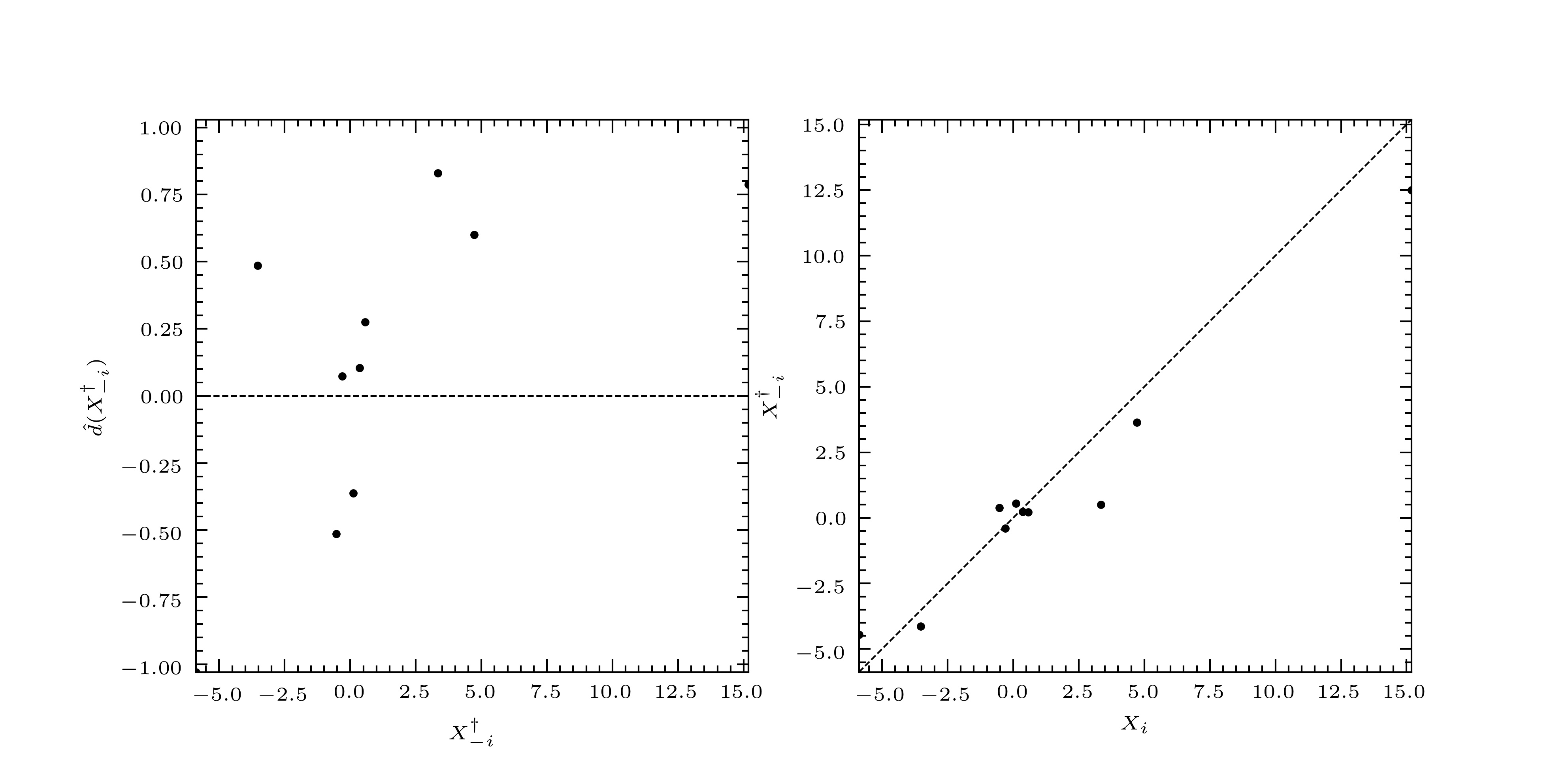
pymimic.plot.diagnostic(xtrain, residuals, var_residuals, figsize=3.3071, 1.6535, xlabel=None, ylabel=None, xlims=None, ylims=None, xticks=None, yticks=None, ticks_kwargs={}, plot_kwargs={}, scatter_kwargs={}, gridspec_kwargs={})[source]¶ Return diagnostic plots for a linear predictor
Returns a two-panel plot consisting of (1) the standardized leave-one-out residuals against the leave-one-out predictions, and (2) the leave-one-out predictions against their true values.
- Parameters:
xtrain ((n,) array_like) – Training output.
residuals ((n,) array_like) – Leave-one-out residuals.
var_residuals ((n,) array_like) – Variances of the leave-one-out residuals.
figsize ((2,) array_like) – Figure size, in the form (width, height).
xlabel ((dim,) array_like, optional) – Labels for \(x\) axes.
ylabel ((dim,) array_like, optional) – Labels for \(y\) axes.
xticks ((dim,) array_like, optional) – Position of \(x\)-ticks for each \(x\)-axis.
yticks ((dim,) array_like, optional) – Position of \(y\)-ticks for each \(y\)-axis.
ticks_kwargs (dict, optional) – Keyword arguments to be passed to
matplotlib.axis.Axis.set_xticks()andmatplotlib.axis.Axis.set_yticks()plot_kwargs (dict, optional) – Keyword arguments to be passed to
matplotlib.pyplot.plot().scatter_kwargs (dict, optional) – Keyword arguments to be passed to
matplotlib.pyplot.scatter().plot_kwargs – Keyword arguments to be passed to
matplotlib.pyplot.plot().gridspec_kwargs (dict) – Keyword arguments to be passed to
matplotlib.pyplot.subplots().
- Returns:
fig – Matrix of plots.
- Return type:
matplotlib.figure.Figure
See also
matplotlib.figure.Figure()Matplotlib’s Figure class.
matplotlib.pyplot.subplots()Matpotlib’s subplots function
matplotlib.pyplot.scatter()Matplotlib’s scatter function.
Example
First fit a curve to a sample of the Forrester function.
>>> ttrain = np.linspace(0., 1., 10)
>>> xxtrain = mim.testfunc.forrester(ttrain)
>>> blup = mim.Blup(ttrain, xtrain, args=(60., 40.))
Now make diagnostic plots using the LOO residuals and their variances.
>>> mim.plot.diagnostic(xtrain, *blup.loocv)
>>> import matplotlib.pyplot as plt
>>> plt.show()
-
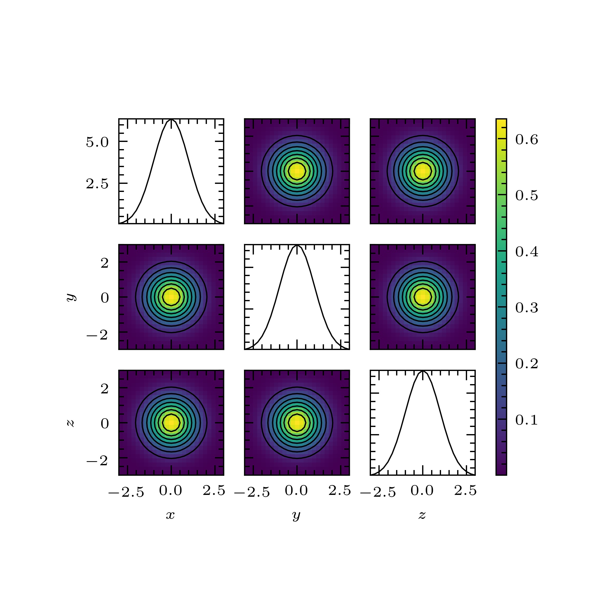
pymimic.plot.plot(Z, extent, figsize=3.3071, 3.3071, xlabel=None, ylabel=None, label_kwargs={}, xticks=None, yticks=None, ticks_kwargs={}, imshow=True, imshow_kwargs={}, contour=True, contour_kwargs={}, cbar=True, cbar_kwargs={}, gridspec_kwargs={})[source]¶ Return plot of the one- and two-dimensional sums of an array.
- Parameters:
Z ((n, dim) array_like) – Sample of function to be plotted.
extent ((2, dim) array) – Limits of the data for each subplot.
figsize ((2,) array_like, optional) – Figure size, in the form (width, height).
xlabel ((dim,) array_like, optional) – Labels for \(x\) axes.
ylabel ((dim,) array_like, optional) – Labels for \(y\) axes.
label_kwargs (dict, optional) – Keyword arguments to be passed to
matplotlib.axis.Axis.set_xlabel()xticks ((dim,) array_like, optional) – Position of \(x\)-ticks for each \(x\)-axis.
yticks ((dim,) array_like, optional) – Position of \(y\)-ticks for each \(y\)-axis.
ticks_kwargs (dict, optional) – Keyword arguments to be passed to
matplotlib.axis.Axis.set_xticks()andmatplotlib.axis.Axis.set_yticks()imshow (bool, optional) – If
Truedisplay heatmap on off-diagonal axes. Default isTrue.imshow_kwargs (dict, optional) – Keyword arguments to be passed to matplotlib.pyplot.imshow.
contour (bool, optional) – If
Truedisplay contours on off-diagonal axes. Default isTrue.contour_kwargs (dict, optional) – Keyword arguments to be passed to
matplotlib.pyplot.contour().cbar (bool, optional) – If
Truedisplay colour bar. Default isTrue.cbar_kwargs (dict) – Keyword arguments to be passed to
matplotlib.pyplot.colorbar().gridspec_kwargs (dict) – Keyword arguments to be passed to
matplotlib.pyplot.subplots().
- Returns:
fig – Matrix of plots.
- Return type:
matplotlib.figure.Figure
See also
matplotlib.figure.Figure()Matplotlib’s Figure class.
matplotlib.pyplot.imshow()Matplotlib’s imshow function.
matplotlib.pyplot.contour()Matplotlib’s contour function.
Notes
The function
plot()can be used to plot the one- and two-dimensional marginalizations of a probability density function or likelihood function. It can also be used, in a rough-and-ready way, to visualize functions of many variables.Each panel of the plot is produced by summing over the unshown dimensions.
The matrix of axes is generated using
matplotlib.pyplot.subplots(). Heat maps are generated usingmatplotlib.pyplot.imshow(). Contours are generated usingmatplotlib.pyplot.contour().Example
Generate and plot a sample of a three-dimensional Gaussian.
>>> import scipy as sp
>>> bounds = [[-3., 3.], [-3., 3.], [-3., 3.]]
>>> x = mim.design(bounds=bounds, method="regular", n=25)
>>> z = sp.stats.multivariate_normal.pdf(x, mean=np.zeros(3), cov=np.eye(3))
>>> z = z.reshape(25, 25, 25)
>>> mim.plot.plot(z, bounds, xlabel=["$x$", "$y$", "$z$"], ylabel=["", "$y$", "$z$"], contour_kwargs={"colors":"k",})
>>> plt.show()
pymimic.testfunc module
A suite of test functions
This module provides several test functions for use in generating illustrative training data (parameters
ttrainandxtrainin the classespymimic.emulator.Blpandpymimic.emulator.Blup).-
pymimic.testfunc.branin(x, y)[source]¶ Return the value of the Branin function for given argument
The Branin function [B72] is the function \(f: \mathbf{R} \times \mathbf{R} \longrightarrow \mathbf{R}\) given by
\[f(x, y) = a (y - bx^2 + cx - d)^2 + e(1 - f) \cos x + e,\]where \(a = 1\), \(b = 5.1 / (4 \pi^2)\), \(c = 5 / \pi\), \(d = 6\), \(e = 10\), \(f = 1 / (8 \pi)\). When used as a test function for optimization its domain is typically restricted to the region \([-5, 10] \times [0, 15]\). In this region the function has three global minima, at \((x, y) = (-\pi, 12.275)\), \((\pi, 2.275)\), and \((9.425, 2.475)\), where it takes the value \(0.398\).
- Parameters:
x ((n,) array_like) – First argument of the function.
y ((n,) array_like) – Second argument of the function.
- Returns:
res – Value of the Branin function.
- Return type:
(n,) ndarray
Example
Single pair of arguments:
>>> mim.testfunc.branin(-np.pi, 12.275)
0.39788736
Multiple pairs of arguments, as two lists:
>>> x = [-np.pi, np.pi, 9.425]
>>> y = [12.275, 2.275, 2.475]
>>> mim.testfunc.branin(x, y)
array([0.39788736, 0.39788736, 0.39788763])
Multiple pairs of elements, as a meshgrid object:
>>> x = np.linspace(-5., 10.)
>>> y = np.linspace(0., 15.)
>>> xx, yy = np.meshgrid(x, y)
>>> mim.testfunc.branin(xx, yy)
array([[308.12909601, 276.06003083, ... ,  10.96088904],
       ...
       [ 17.50829952,  11.55620801, ... , 145.87219088]])
References
[B72]Branin, F.H. 1972. 'Widely convergent method for finding multiple solutions of simultaneous nonlinear equations' in IBM Journal of Research and Development, 16 (5): 504–22. Available at http://www.doi.org/10.1147/rd.165.0504.
-
pymimic.testfunc.forrester(x)[source]¶ Return the value of the Forrester function for given argument
The Forrester function [F08] is the function \(f: \mathbf{R} \longrightarrow \mathbf{R}\) given by
\[f(x) = (6x - 2)^2 \sin(12x - 4).\]When used as a test function for optimization its domain is typically restricted to the region \([0, 1]\).
- Parameters:
x ((n,) array_like) – Argument of the function.
- Returns:
res – Value of the Forrester function.
- Return type:
(n,) ndarray
Example
Single argument:
>>> mim.testfunc.forrester(0.5)
0.9092974268256817
Multiple arguments:
>>> t = np.linspace(0., 1., 10)
>>> mim.testfunc.forrester(t)
array([ 3.02720998, -0.81292911, ... , 15.82973195])
References
[F08]Forrester, A., Sobester, A., and A. Keane. 2008. Engineering design via surrogate modelling: a practical guide. Wiley.
-
pymimic.testfunc.gp(t, covfunc=<function squared_exponential>, args=())[source]¶ Return a realization a centred Gaussian random process
- Parameters:
t ((n, d) array_like) – Argument of the function.
covfunc (callable) – Covariance kernel of the Gaussian random process
args (tuple) – Extra arguments to be passed to the covariance kernel,
covfunc.
- Returns:
res – Sample of a realization of a centred Gaussian random process.
- Return type:
(n,) ndarray
Example
One one-dimensional argument:
>>> mim.testfunc.gp(1., mim.kernel.squared_exponential, (1., 1.))
array([0.83792787])
Multiple one-dimensional arguments:
>>> t = np.linspace(0., 1.)
>>> mim.testfunc.gp(t, mim.kernel.squared_exponential, (1., 1.))
array([-0.9635262 , -0.9457061 , ... , -0.25218523])
One two-dimensional argument:
>>> mim.testfunc.gp([[0., 1.]], mim.kernel.squared_exponential, (1., 1., 1.))
array([0.59491435])
Multiple two-dimensional arguments:
>>> t = mim.design.design([[0., 1.], [0., 1.]], "regular", 10)
>>> mim.testfunc.gp(t, mim.kernel.squared_exponential, (1., 1., 1.)).reshape(10, 10)
array([[-0.9635262 , -0.9457061 , ... , -0.89178485],
       ...
       [-0.29947984, -0.28774821, ... , -0.25218523]])