Validation¶

We must always test the performance of a linear predictor, a procedure known as 'validation'. In leave-\(p\)-out cross-validation, instead of using a validation set distinct from \(X\), we partition \(X\) into a set containing \(p\) elements, \(X_{P}\), and a set containing \(n - p\) elements, \(X_{\bar{P}}\). We construct a predictor for each \(X_{i} \in X_{P}\) based on \(X_{\bar{P}}\), namely \(\hat{Z}_{i}\).

Commonly, \(p = 1\). We denote the \(j\)-th leave-one-out linear predictor of \(X_{j}\) by \(\hat{X}_{- j}\). Similarly we denote the \(j\)-th leave-one-out linear predictor of \(X_{j}\) by \(\hat{X}_{- j}\). The leave-one-out cross-validation linear predictor residual is

\[e(\hat{Z}_{- j}) = Z_{j} - \hat{Z}_{- j},\]

and the standardized leave-one-out cross-validation linear predictor residual is

\[d(\hat{Z}_{- j}) = \dfrac{Z_{j} - \hat{Z}_{- j}}{\sqrt{\operatorname{var}(\hat{Z}_{- j})}}.\]

The behaviour of the observed predictor residuals should be consistent with the assumptions we have made about their distribution.

A good summary statistic is provided by the leave-one-out cross-validation score

\[R^{2} = \dfrac{1}{n}\sum_{i}d(\hat{Z}_{- i})^{2}.\]

PyMimic and validation¶

The LOO residuals and their variances are stored as the attribute loocv belonging to the classes BLP and BLUP. The module mim.plot contains the function diagnostic(), which plots (1) the standardized LOO residuals against the LOO predictions and (2) the LOO predictions against against their true values.

Let us validate the predictor we used in fitting a curve to a noisy sample of the Branin function.

Generate the sample.

>>> import pymimic as mim
>>> bounds = [[-5., 10.], [0., 15.]]
>>> ttrain = mim.design(bounds)
>>> xtrain = mim.testfunc.branin(*ttrain.T) + 10.*np.random.randn(20)

Then create a BLUP object.

>>> blup = mim.Blup(ttrain, xtrain, 10.**2.)
>>> blup.opt()
   direc: array([[1., 0., 0.],
       [0., 1., 0.],
       [0., 0., 1.]])
     fun: 169.40632097688868
 message: 'Optimization terminated successfully.'
    nfev: 146
     nit: 3
  status: 0
 success: True
       x: array([1.57069249, 0.08700307, 0.01322379])

Now compute the the LOO prediction residuals and their variances.

>>> blup.loocv
(array([ 51.2065913 , -25.12770775,  19.39411263, -26.15146519,
         4.46734306, -15.74786283,  23.69329757,   4.60761066,
        11.70811329, -17.17898489,   2.20727369, -31.45013478,
        31.868371  ,  11.49837525,  16.08973502, -11.11629167,
       -10.78144937, -18.14250451,  -3.22056033,   8.3367355 ]),
 array([999.76676916, 904.42982646, 888.29496818, 382.93648001,
        817.77977058, 279.85877825, 267.51340703, 712.60225493,
        267.13441485, 426.51943097, 426.51943097, 267.13441485,
        712.60225493, 267.51340703, 279.85877825, 817.77977058,
        382.93648001, 888.29496818, 904.42982646, 999.76676916]))

Also compute the LOOCV validation score.

>>> blp.R2
9992.090822466882

Now plot the results.

>>> mim.plot.diagnostic(xtrain, *blup.loocv)

The result is show in Fig. 3.

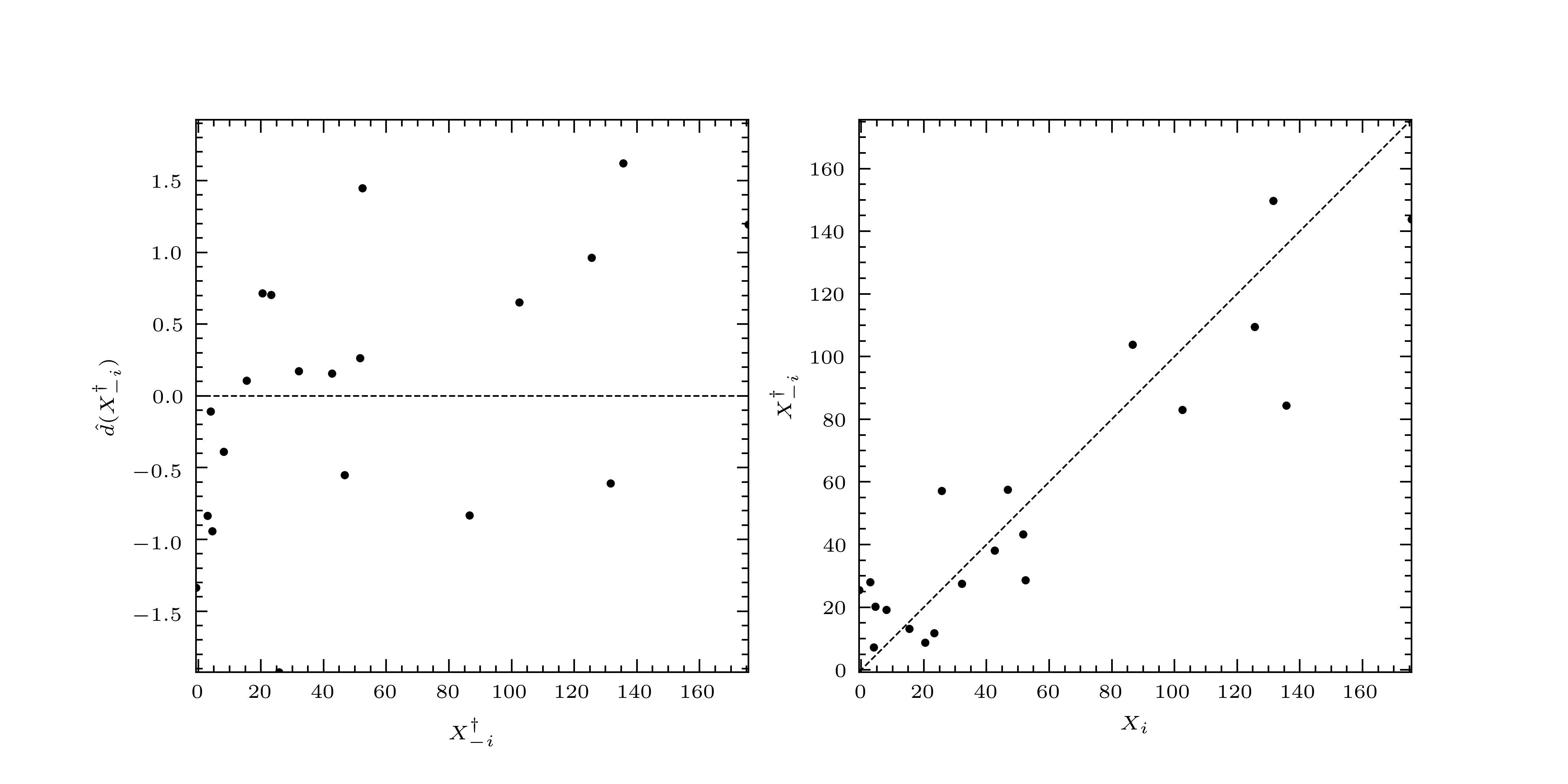
../_images/branin_diagnostic.jpg — Fig. 4 Left: the standardized LOO residuals plotted against the LOO predictions. Right: the LOO predictions plotted against their true values.¶

The standardized LOO residuals are small and randomly distributed. When plotted against their true values, the predictions lie around the diagonal. So we say, in this case, that the predictor has passed validation, and that we may trust the fitted curve and its associated prediction interval.