Linear prediction¶

The two flavours of linear prediction¶

A linear predictor for a random variable \(Z\) based on a random process \(X := \{X_{t}\}_{t \in T}\) is a linear combination of the elements of \(X\). By denoting this predictor \(\hat{Z}\) we have that

\[\hat{Z} = \sum_{i = 1}^{n}a_{t}X_{t}.\]

If the random vector \((Z, X)\) is second order we may form the best linear predictor (BLP) by choosing the set of coefficients, \((a_{t})_{t \in T}\), so as to minimize the mean-squared error, \(\operatorname{E}((Z - \hat{Z})^{2})\).

We may further impose the constraint that the expected values of \(Z\) and \(\hat{Z}\) are equal, i.e. that \(\operatorname{E}(\hat{Z}) = \operatorname{E}(Z)\). In order to do this, we work under the assumption that \(\operatorname{E}\) is an element of a finite-dimensional space of functions, \(F\). We then minimize the mean-squared error \(\operatorname{E}((Z - \hat{Z})^{2})\) subject to the constraint that \(\operatorname{E}_{f}(\hat{Z}) = \operatorname{E}_{f}(Z)\) for all \(\operatorname{E}_{f} \in F\). We call this the best linear unbiased predictor (BLUP) [G62].

Now extend \(T\) so that, by writing \(Z = X_{t_{0}}\), it also indexes both \(X\) and \(Z\), and consider the the random random process \((X_{t_{0}}, X)\). The mean-value function is

\[ \begin{align}\begin{aligned}m: T &\longrightarrow \mathbf{R}\\t &\longmapsto \operatorname{E}(X_{t}),\end{aligned}\end{align} \]

second moment kernel is

\[ \begin{align}\begin{aligned}r: T \times T &\longrightarrow \mathbf{R}\\(s, t) &\longmapsto \operatorname{E}(X_{s}X_{t}),\end{aligned}\end{align} \]

and the covariance kernel is

\[ \begin{align}\begin{aligned}k: T \times T &\longrightarrow \mathbf{R}\\(s, t) &\longmapsto \operatorname{cov}(X_{s}, X_{t}).\end{aligned}\end{align} \]

The best linear predictor¶

Let \(X := \{X_{t}\}_{t \in T}\) be a random process (considered as a column vector) with finite index set \(T\) and second-moment kernel \(r\). Let \(Z\) be a random variable to which the second-moment kernel extends by writing \(Z = X_{t_{0}}\). The best linear predictor (BLP) of \(Z\) based on \(X\) is

\[Z^{*} = \sigma{}^{\mathrm{t}}K^{-1}X\]

where \(\sigma := (r(t_{*}, t_{i}))_{i}\) and \(K := (r(t_{i}, t_{j}))_{ij}\). The mean-square error of the BLP is

\[\operatorname{MSE}(Z^{*}) = r(t_{0}, t_{0}) - \sigma^{\mathrm{t}}K^{-1}\sigma.\]

Given a realization of \(X\), namely \(x\), then we may compute the realization of \(Z^{*}\), namely \(z^{*}\), by making the substitution \(X = x\).

The best linear unbiased predictor¶

Now let \(k\) be the covariance kernel for \(X\), and let \(Z\) be a random variable to which the covariance kernel extends by writing \(Z = X_{t_{0}}\). Let \((f_{i})_{i}\) be a basis for the space of possible mean-value functions for \(Z\). The best linear unbiased predictor (BLUP) of \(Z\) based on \(X\) is

\[Z^{\dagger} = \Theta^{\dagger} + \sigma^{\mathrm{t}}K^{-1}\mathrm{D}\]

where \(\sigma := (k(t_{0}, t_{i}))_{i}\), \(K := (k(t_{i}, t_{j}))_{ij}\), \(\Theta^{\dagger} = \phi^{\mathrm{t}}\mathrm{B}\), \(\mathrm{D} := X - \Phi\mathrm{B}\), and where \(\phi = (f_{i}(t_{0}))_{i}\), \(\Phi := (f_{i}(t_{j}))_{ij}\), and \(\mathrm{B} := (\Phi^{\mathrm{t}}K^{\,-1}\Phi)^{-1}\Phi^{\mathrm{t}}K^{\,-1}X\). Note that \(\Theta^{\dagger}\) is the best linear unbiased unbiased estimator (BLUE) of the mean of \(Z\), and \(\Phi\mathrm{B}\) is the tuple of best linear estimators of the the elements of \(X\). The mean-square error of the BLUP is

\[\operatorname{MSE}(Z^{\dagger}) = k(t_{0}, t_{0}) - \sigma^{\mathrm{t}}K^{-1}\sigma + (\phi^{\mathrm{t}} - \sigma^{\mathrm{t}}K^{-1}\Phi)(\Phi^{\mathrm{t}}K^{\,-1}\Phi)^{-1}(\phi - \Phi^{\mathrm{t}}K^{-1}\sigma).\]

Again, given a realization of \(X\), namely \(x\), then we may compute the realization of \(Z^{\dagger}\), namely \(z^{\dagger}\), by making the substitution \(X = x\).

Prediction intervals¶

When forming a prediction interval for \(Z\) we are interested in the quantity \(Z - (\hat{Z} - \operatorname{bias}(\hat{Z}))\). Suppose that we have a model for the distribution of this quantity, and, furthermore, that we have a pair of \(\gamma\) critical values for this model, \(c_{1}\) and \(c_{2}\). Then a \(\gamma\) prediction interval for \(Z\) is

\[[\hat{Z} - \operatorname{bias}(\hat{Z}) + c_{1}\sqrt{\operatorname{var}(Z - \hat{Z})}, \hat{Z} - \operatorname{bias}(\hat{Z}) + c_{2}\sqrt{\operatorname{var}(Z - \hat{Z})}]\]

where the bias-variance decomposition gives

\[\operatorname{MSE}(\hat{Z}) = \operatorname{var}(Z - \hat{Z}) + (\operatorname{bias}(\hat{Z}))^{2}.\]

In the case that \(\hat{Z}\) is the BLUP of \(Z\) then \(\operatorname{bias}(\hat{Z}) = 0\). However, in the case that \(\hat{Z}\) is the BLP of \(Z\) we do not in general know \(\operatorname{bias}(\hat{Z})\).

Furthermore, we do not, in general, have a model for the distribution of \(Z - (\hat{Z} - \operatorname{bias}(\hat{Z}))\) in either the case of the BLP or the BLUP. We have two options: (1) assume an arbitrary model for distribution (typically Gaussian), or (2) use either Chebyshev’s inequality or the Vysochanskij–Petunin inequality to construct bounds for the prediction interval. In the second case, we can construct the worst-case prediction interval, given by

\[[\hat{Z} - \operatorname{bias}(\hat{Z}) + \lambda\sqrt{\operatorname{var}(Z - \hat{Z})}, \hat{Z} - \operatorname{bias}(\hat{Z}) + \lambda\sqrt{\operatorname{var}(Z - \hat{Z})}]\]

at confidence level \(\gamma = 1 - 4/(9\lambda^{2})\) (Vysochanskij–Petunin inequality, case of unimodal distribution) or \(\gamma = 1 - 1/\lambda^{2}\) (Chebyshev’s inequality, general case).

Known and unknown quantities¶

We imagine the following three states of knowledge.

We know the second-moment kernel but not the mean-value function or covariance kernel. In this situation the BLP and the MSE of the BLP are known, but the bias of the BLP, the BLUP and the MSE of the BLUP are not known.

We know the covariance kernel but not the mean-value function or second-moment function. In this situation the BLUP and MSE of the BLUP are known, but the BLP, the MSE of the BLP, and the bias of the BLP are not known.

We know the mean-value function and either (equivalently, both) the second-moment kernel or covariance kernel. In this situation the BLP, the MSE of the BLP, and the bias of the BLP, along with the BLUP and the MSE of the BLUP, are all known.

In case 3 we may centre \(Z\) and \(X\) by subtracting \(\mathrm{E}(Z)\) and \(\mathrm{E}(X)\) respectively. Furthermore, we may choose the very simplest space of pseudoexpectation functions, \(F\), namely the space generated by the single element \(\mathrm{E}\). The second and third terms in the BLUP formula then vanish, as does the third term in its MSE formula. For centred random variables, the second-moment kernel and covariance kernel are identical. Therefore, in this case, the BLP and the BLUP coincide.

Linear prediction and curve fitting¶

We may use linear prediction for the purposes of curve fitting if we adopt the conceit that a curve, \(z\), is the realization of a random process \(Z = (Z_{t})_{t \in T}\), indexed by the domain of \(z\), namely \(T \in \mathbf{R}^{d}\) for some \(d\). Let \((Z_{t_{i}})_{i \le n}\) be a finite sample of \(Z\), let \((H_{i})_{i \le n}\) be a centred random vector, and consider the random vector \(X := (Z_{t_{i}} + H_{i})_{i \le n}\), which we view as a sample of \(Z\) contaminated by noise. We can the find a linear predictor of any element of \(Z\) based on \(X\). The set of all such predictors, \((\hat{Z}_{t})_{t \le T}\) is called a 'linear smoother'. In the case that \(H_{i}\) is 0 for all \(i\) such a smoother is called a 'linear interpolator'.

PyMimic and linear prediction¶

Suppose that we have some data, which, for the sake of concreteness, we take to be a noisy sample of the two-variable Branin function, \(x: [-5, 10] \times [0, 15] \longrightarrow \mathbf{R}\), given by

\[x(t_{0}, t_{1}) = a (t_{1} - bt_{0}^2 + ct_{0} - r)^2 + s(1 - t) \cos t_{0} + s,\]

where \(a = 1\), \(b = 5.1 / (4 \pi^2)\), \(c = 5 / \pi\), \(r = 6\), \(s = 10\), and \(t = 1 / (8 \pi)\).

The process is two-fold. First we must generate a set of training data for the function. Second we must use these training data to predict the value \(x(t_{0}^{*}, t_{1}^{*})\) for arbitrary \((t_{0}^{*}, t_{1}^{*}) \in [-5, 10] \times [0, 15]\). We may do this using the BLP or the BLUP. PyMimic provides the classes Blp and Blup for these purposes.

We may generate the training data using the function design(). By default this returns an experimental design of sample size \(10d\), where \(d\) is the length of the training input, using Latin-hypersquare sampling. (See Experimental designs for an overview of design generation in PyMimic.)

>>> bounds = [[-5., 10.], [0., 15.]]
>>> ttrain = mim.design(bounds)

Generate the training output. The Branin function is included in PyMimic’s suite of test functions, testfunc, so we do not need to define it ourselves.

>>> import pymimic as mim
>>> xtrain = mim.testfunc.branin(*ttrain.T) + 10.*np.random.randn(20)

We have here used homoskedastic errors (i.e. errors of equal variance). But note that heteroskedastic errors may also be used.

Curve fitting using the BLP¶

Let us predict values of the Branin function using the BLP. We will use a squared-exponential covariance kernel, which is included in the module kernel. (See Covariance and second-moment kernels for details on specifying positive-definite kernels for use with PyMimic.) First create an instance of the class Blp, specifying the covariance kernel using the keyword kernel, and then optimizing its parameters.

>>> blp = mim.Blp(ttrain, xtrain, 10.**2., covfunc=mim.kernel.squared_exponential)
>>> blp.opt()
   message: Optimization terminated successfully.
success: True
 status: 0
    fun: 157.22085324793372
      x: [ 1.571e+00  1.751e-02  5.377e-03]
    nit: 5
  direc: [[ 0.000e+00  0.000e+00  1.000e+00]
          [ 0.000e+00  1.000e+00  0.000e+00]
          [ 3.242e-05 -6.780e-03 -3.954e-03]]
   nfev: 255

Now generate the values of \(t\) for which we wish to predict the Branin function.

>>> t = mim.design(bounds, "regular", 50)

And compute the predictions and their mean-squared errors by calling the method xtest().

>>> x, mse = blp.xtest(t)
>>> x
[239.14432682 221.71949142 202.8843214  ... 105.88388496  93.78647069
  82.483802  ]
>>> mse
[1017.85925982  772.13821831  583.09152623 ...  583.09152623  772.13821831
 1017.85925982]

We may construct a biased prediction interval as follows.

>>> x + (- 3.*np.sqrt(mse), 3.*np.sqrt(mse))
[[143.43260685 138.35736594 130.44245688 ...  33.44202043  10.42434521
  -13.22791796]
 [334.85604678 305.0816169  275.32618593 ... 178.32574948 177.14859617
  178.19552196]]

Now plot the predictions.

>>> import matplotlib.pyplot as plt
>>> im = plt.imshow(x.reshape(50, 50), extent=[-5., 10., 0., 15.], origin="lower", vmin=-25., vmax=250.)
>>> plt.contour(np.linspace(-5., 10.), np.linspace(0., 15.), x.reshape(50, 50), levels=np.linspace(-25., 250., 12))
>>> x_branin = mim.testfunc.branin(*t.T)
>>> plt.contour(np.linspace(-5., 10.), np.linspace(0., 15.), x_branin.reshape(50, 50), linestyles="dashed", levels=np.linspace(-25., 250., 12))
>>> plt.scatter(ttrain.T[0], ttrain.T[1])
>>> plt.colorbar(im)
>>> plt.show()

The result is show in Fig. 3.

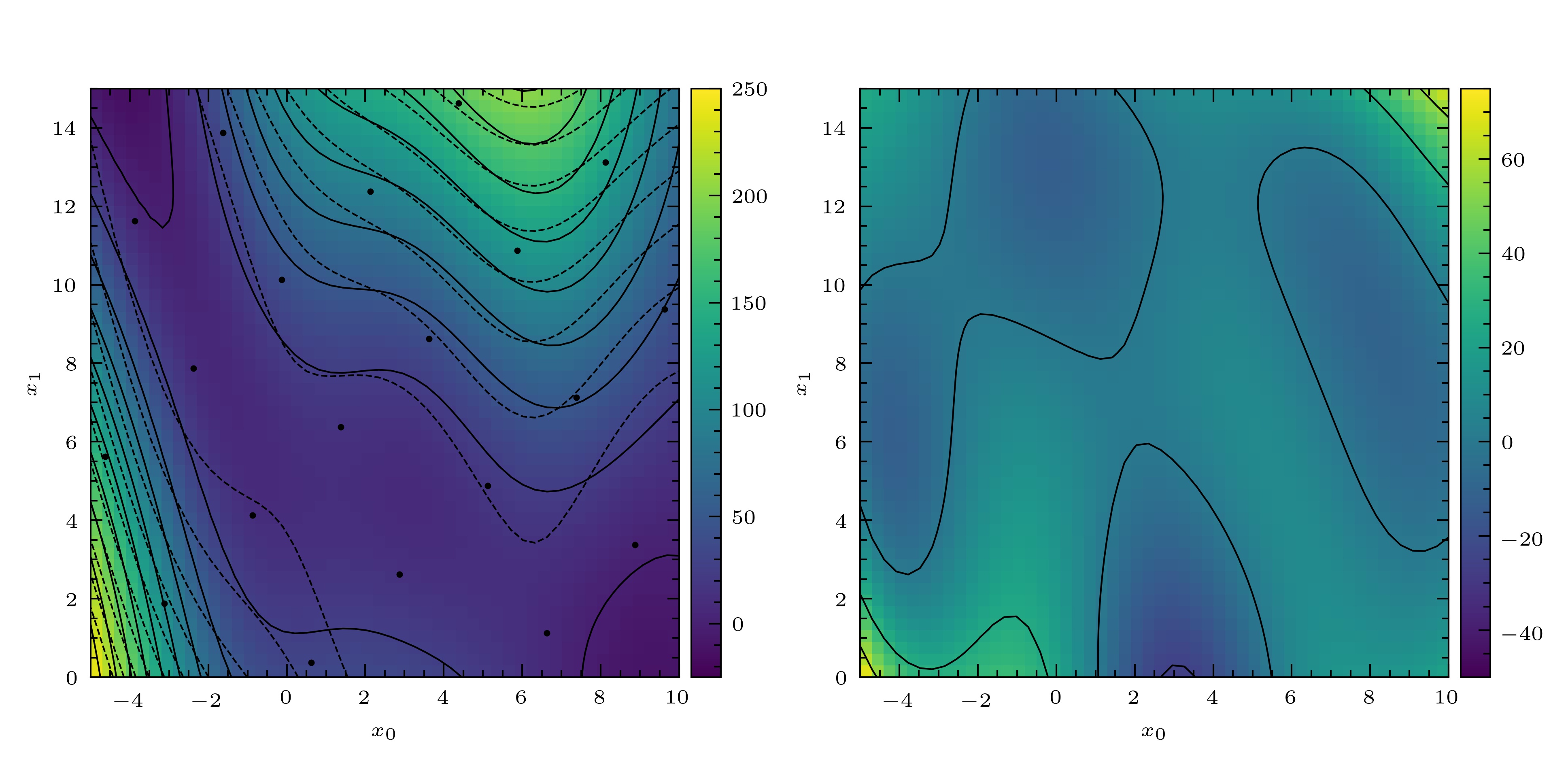
../_images/branin_blp.jpg — Fig. 3 Left: the Branin function (dashed lines), a noisy sample of the Branin function (filled circles) and curve fitted to this samle using the BLP (solid line, colour map). Right: residuals of the fitted curve.¶

Note that the covariance matrix, \(K\), is available as the attribute K.

>>> blp.K
[[1.61000000e+04 1.33043190e+04 1.37262145e+04 1.27726667e+04
21784059e+03 9.02468610e+03 6.49780042e+03 4.69293165e+03
78126070e+03 2.10656250e+03 1.61945346e+03 1.00963484e+03
35216671e+02 3.56136025e+02 1.71796863e+02 9.24547191e+01
99098811e+01 1.86289906e+01 1.06713518e+01 4.45738714e+00]
 [1.33043190e+04 1.61000000e+04 1.01991815e+04 1.37262145e+04
27726667e+04 8.66648877e+03 9.02468610e+03 4.02714413e+03
69293165e+03 3.78126070e+03 1.79604805e+03 1.61945346e+03
00963484e+03 5.10460241e+02 3.56136025e+02 1.18417794e+02
24547191e+01 4.99098811e+01 1.76646020e+01 1.06713518e+01]
 ...
 [4.45738714e+00 1.06713518e+01 1.86289906e+01 4.99098811e+01
24547191e+01 1.71796863e+02 3.56136025e+02 4.35216671e+02
00963484e+03 1.61945346e+03 2.10656250e+03 3.78126070e+03
69293165e+03 6.49780042e+03 9.02468610e+03 8.21784059e+03
27726667e+04 1.37262145e+04 1.33043190e+04 1.61000000e+04]]

Curve fitting using the BLUP¶

Curve fitting with the BLUP differs from curve fitting with the BLP only insofar as we must also specify a basis for the space of mean-value functions. We will use a basis consisting of the constantly one function, which is included in the module basis. (See Bases for the space of mean-value functions for details on specifying basis functions for use with PyMimic.) First create an instance of the class Blup, specifying the basis using the keyword basis. Again, we must optimize the parameters of the covariance kernel.

>>> blup = mim.Blup(ttrain, xtrain, 10.**2., covfunc=mim.kernel.squared_exponential, basis=mim.basis.const())
>>> blup.opt()
message: Optimization terminated successfully.
success: True
 status: 0
    fun: 155.50248314797585
      x: [ 1.571e+00  2.250e-02  8.333e-03]
    nit: 5
  direc: [[ 1.238e-04 -1.030e-02 -5.152e-03]
          [ 0.000e+00  1.000e+00  0.000e+00]
          [ 2.212e-06 -3.640e-04 -2.789e-04]]
   nfev: 231

Now proceed as for the case of the BLP.

>>> x, mse = blup.xtest(t)
>>> x
[253.14107798 233.17364885 212.21929952 ... 115.21886307 105.24062812
  96.48055316]
>>> mse
[1067.61478274  805.45884088  605.2231572  ...  605.2231572   805.45884088
 1067.61478274]

Since the BLUP is unbiased we may construct unbiased prediction intervals.

>>> x + (-3.*np.sqrt(mse), 3.*np.sqrt(mse))
[[155.11795293 148.03182852 138.41544857 ...  41.41501212  20.09880779
   -1.54257189]
 [351.16420303 318.31546917 286.02315047 ... 189.02271402 190.38244844
  194.50367821]]

Again, the covariance matrix, \(K\), is available as an attribute, as are \(\mathrm{B}\) and \(\mathrm{D}\).

>>> blup.Beta
[130.71751617]
>>> blup.Delta
[   4.9222105  -127.80794541  -28.26712086 -131.42748909  -88.10486623
 -126.24457174  -78.34413201  -98.63325872 -110.28064121  -44.10783169
 -115.34168051 -104.97364037   44.89235465 -107.46833086   -5.18267962
 -122.66981728  -83.95459423    0.83137284 -126.72769242  -79.06152086]

References¶

[G62]

Goldberger, A. S. 1962. 'Best linear unbiased prediction in the generalized linear regression model' in Journal of the American Statistical Association, 57 (298): 369–75. Available at https://www.doi.org/10.1080/01621459.1962.10480665.

[S89]

Sacks, J., Welch, W. J., Mitchell, T.J., and H. P. Wynn. 1989. ‘Design and analysis of computer experiments’ in Statistical science, 4 (4): 409–23. Available at https://doi.org/10.1214/ss/1177012413.